💡 Unit V: Dynamic Programming
Design and Analysis of Algorithms (MIT121)
Second Semester — Master of Information Technology
§ 5.1 — Greedy vs Dynamic Programming
🆚 Greedy vs Dynamic Programming
Both Greedy Algorithms and Dynamic Programming tackle optimization problems — finding the best solution under given constraints. Yet they differ fundamentally in strategy, guarantee, and when to apply each.
✅ Greedy Approach
- Makes locally optimal choice each step
- Never re-evaluates past decisions
- Usually O(n log n) or O(n)
- Works only if greedy-choice property holds
- Uses O(1) extra memory
- Examples: Fractional Knapsack, Huffman, Prim's MST
🔄 Dynamic Programming
- Explores all choices systematically
- Stores and reuses subproblem results
- Usually O(n²) to O(n³) time
- Correct when optimal substructure holds
- Requires O(n²) memory for DP table
- Examples: 0/1 Knapsack, Edit Distance, Matrix Chain
| Criterion | Greedy | Dynamic Programming |
|---|---|---|
| Decision making | Locally optimal per step | Globally optimal via all subproblems |
| Subproblem reuse | Each subproblem solved once (no overlap) | Overlapping subproblems stored & reused |
| Correctness | Only when greedy-choice property holds | Always correct if optimal substructure holds |
| Time complexity | Generally lower | Polynomial but higher (O(n²) or O(n³)) |
| Space complexity | O(1) extra space | O(n²) for DP table |
| Backtracking | Not needed | Reconstruct solution from stored table |
Fractional Knapsack: Items can be divided. Greedy (highest v/w ratio first) gives optimal in O(n log n). ✔
0/1 Knapsack: Items cannot be divided. Greedy fails — choosing the locally best item can block better combinations. DP evaluates all item-capacity combinations → guarantees global optimum. ✔
Example: Items = {(wt=10,val=60),(wt=20,val=100),(wt=30,val=120)}, W=50. Greedy by ratio picks item1+item2 = 160. DP optimal = item2+item3 = 220. Greedy fails here!
Rule of Thumb: If the local best choice always leads to the global optimum → Greedy. If local choices can lead to globally suboptimal outcomes → Dynamic Programming.
§ 5.2 — Recursion vs Dynamic Programming
🔁 Recursion vs Dynamic Programming
Naive recursion and DP can solve many of the same problems, but plain recursion without result-caching recomputes identical subproblems exponentially many times. DP eliminates this by ensuring each subproblem is solved exactly once.
The Fibonacci Case Study
The Fibonacci sequence is the simplest yet most illustrative example of DP's advantage over plain recursion.
PYTHON — Naive Recursion — O(2ⁿ) time
def fib_naive(n):
    if n <= 1: return n
    return fib_naive(n-1) + fib_naive(n-2)
# fib(5): fib(2) called 3×, fib(3) called 2× — exponential recomputation!
PYTHON — Dynamic Programming — O(n) time, O(n) space
def fib_dp(n):
    if n <= 1: return n
    dp = [0] * (n + 1)
    dp[1] = 1
    for i in range(2, n + 1):
        dp[i] = dp[i-1] + dp[i-2]  # each value computed ONCE
    return dp[n]

# Further optimized: O(1) space using two variables
def fib_opt(n):
    a, b = 0, 1
    for _ in range(n): a, b = b, a + b
    return a
           fib(5)
          /       \
      fib(4)      fib(3) 🔴
      /    \       /    \
  fib(3)🔴 fib(2)🔴 fib(2)🔴 fib(1)
  /  \     /  \    /  \
f(2) f(1) f(1) f(0) f(1) f(0)
/  \
f(1) f(0)
Redundant: fib(3)×2 | fib(2)×3 | fib(1)×5 | fib(0)×3
Naive recursion for fib(n) has time complexity O(2ⁿ). DP (bottom-up tabulation) reduces it to O(n) time and O(n) space, or even O(1) space with rolling variables. For n=50: from 10¹⁵ calls → just 50 additions!
When to Prefer DP over Recursion?
- Overlapping Subproblems: The same subproblem appears multiple times in the recursive call tree.
- Optimal Substructure: An optimal solution to the whole problem contains optimal solutions to subproblems.
- Deterministic Subproblems: Given the same inputs, a subproblem always produces the same output — results can safely be cached.
- Polynomial State Space: Total distinct subproblems is polynomial, not exponential — making a table feasible.
§ 5.3 — Elements of Dynamic Programming Strategy
📐 Elements of Dynamic Programming Strategy
To correctly formulate a DP solution, a problem must satisfy two essential structural properties.
Property 1 — Optimal Substructure
How to check: Suppose you have an optimal solution S* to problem P. If the restriction of S* to any subproblem P' arising in S* is also optimal for P' → optimal substructure exists.
Example — Shortest Path: Shortest path from A→C through B: the path A→B within the optimal A→C path must itself be the shortest A→B path. If not, replace it — contradiction! ✔ Optimal substructure holds.
Counterexample — Longest Simple Path: The longest simple path from A→C via B does NOT necessarily use the longest simple A→B sub-path — the overall path must remain simple (no repeated vertices). ✘ No optimal substructure.
Property 2 — Overlapping Subproblems
Unlike Divide & Conquer (which produces independent subproblems), DP applies when subproblems overlap — the same smaller problem is encountered repeatedly during recursion.
DP stores solutions to subproblems in a table (array/hash map). When a subproblem is first solved, its result is stored. All future occurrences simply look up the stored value. Total work = O(distinct subproblems × work per subproblem).
The Four-Step DP Development Process
- Characterize optimal structure: Identify what choices lead to subproblems. Prove optimal substructure.
- Define recurrence: Write the optimal value of a solution recursively in terms of smaller subproblems. Clearly state base cases.
- Compute bottom-up (tabulation): Fill a table from smallest subproblems to largest. Each cell depends only on already-computed cells.
- Reconstruct solution: Use a separate "choice" table to trace back the actual optimal solution (not just the optimal value).
§ 5.4 — Matrix Chain Multiplication (MCM)
🔢 Matrix Chain Multiplication
The Matrix Chain Multiplication problem asks: given a chain of n matrices A₁·A₂·…·Aₙ, find the parenthesization that minimizes the total number of scalar multiplications. Matrix multiplication is associative, so the order of computing products can vary — and this choice dramatically impacts cost.
Why Parenthesization Matters
Matrices: A(10×30), B(30×5), C(5×60)
- (AB)C: AB costs 10×30×5 = 1,500 → then 10×5×60 = 3,000. Total = 4,500
- A(BC): BC costs 30×5×60 = 9,000 → then 10×30×60 = 18,000. Total = 27,000
First parenthesization is 6× cheaper. With many matrices, the difference can be astronomical.
DP Recurrence
Let m[i][j] = minimum scalar multiplications to compute A[i..j].
Step-by-Step: 4 Matrices Example
Given p = [5, 10, 3, 12, 5], meaning A₁(5×10), A₂(10×3), A₃(3×12), A₄(12×5).
PYTHON — Matrix Chain Multiplication (Bottom-Up DP)
def matrix_chain_order(p):
    n = len(p) - 1       # number of matrices
    m = [[0]*n for _ in range(n)]
    s = [[0]*n for _ in range(n)]  # split point table

    for l in range(2, n+1):        # chain length
        for i in range(n - l + 1):
            j = i + l - 1
            m[i][j] = float('inf')
            for k in range(i, j):
                cost = m[i][k] + m[k+1][j] + p[i]*p[k+1]*p[j+1]
                if cost < m[i][j]:
                    m[i][j] = cost
                    s[i][j] = k     # remember split
    return m, s

def print_optimal(s, i, j):
    if i == j: print(f"A{i+1}", end="")
    else:
        print("(", end="")
        print_optimal(s, i, s[i][j])
        print_optimal(s, s[i][j]+1, j)
        print(")", end="")
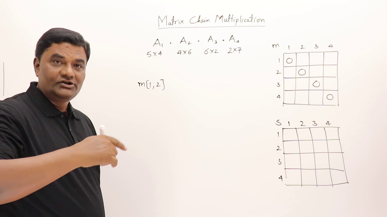
- The number of distinct parenthesizations of n matrices is the (n-1)th Catalan number — exponentially many. DP reduces search to polynomial time.
- The DP table is filled diagonally: first all chains of length 2, then length 3, up to length n.
- The split point table
s[i][j]records which split k gave the minimum, enabling reconstruction of the actual parenthesization. - MCM does NOT actually multiply the matrices — it finds the optimal order for doing so.
§ 5.5 — String Editing (Edit Distance)
📝 Edit Distance (Levenshtein Distance)
The Edit Distance between two strings is the minimum number of single-character edit operations required to transform one string into another. Applications: spell-checking, DNA sequencing, diff tools, NLP.
- Insert: Insert a character into the string
- Delete: Remove a character from the string
- Replace (Substitute): Replace one character with another
DP Formulation
Let dp[i][j] = minimum edits to transform the first i characters of X into the first j characters of Y.
Worked Example: "SUNDAY" → "SATURDAY"
X = "SUNDAY" (len=6), Y = "SATURDAY" (len=8). dp[6][8] = 3 edits
Answer: dp[6][8] = 3 edits (highlighted in gold)
PYTHON — Edit Distance (Bottom-Up DP)
def edit_distance(X, Y):
    m, n = len(X), len(Y)
    dp = [[0]*(n+1) for _ in range(m+1)]
    for i in range(m+1): dp[i][0] = i  # delete all
    for j in range(n+1): dp[0][j] = j  # insert all
    for i in range(1, m+1):
        for j in range(1, n+1):
            if X[i-1] == Y[j-1]:
                dp[i][j] = dp[i-1][j-1]
            else:
                dp[i][j] = 1 + min(
                    dp[i-1][j],   # delete X[i]
                    dp[i][j-1],   # insert Y[j]
                    dp[i-1][j-1]  # replace
                )
    return dp[m][n]

§ 5.6 — 0/1 Knapsack Problem
🎒 0/1 Knapsack Problem
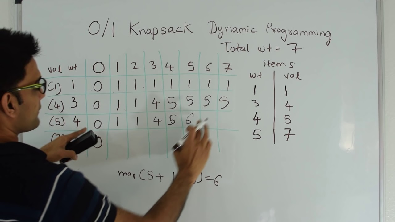
In the 0/1 Knapsack Problem, you have n items each with a weight and value, and a knapsack of capacity W. For each item, you either take it entirely (1) or leave it (0) — no fractions allowed. Find the combination maximizing total value without exceeding capacity.
Output: Maximum value achievable by selecting a subset of items with total weight ≤ W.
DP Recurrence
Let dp[i][w] = maximum value using items 1..i with weight limit w.
Worked Example
Items: (w=2,v=6), (w=2,v=10), (w=3,v=12). Capacity W = 5.
Optimal = 22 (Item 2 + Item 3 = 10+12, weight=5)
PYTHON — 0/1 Knapsack (Bottom-Up DP)
def knapsack_01(weights, values, W):
    n = len(weights)
    dp = [[0]*(W+1) for _ in range(n+1)]
    for i in range(1, n+1):
        for w in range(W+1):
            if weights[i-1] > w:
                dp[i][w] = dp[i-1][w]
            else:
                dp[i][w] = max(dp[i-1][w],
                               values[i-1] + dp[i-1][w - weights[i-1]])
    return dp[n][W]

def get_items(dp, weights, W, n):
    result, w = [], W
    for i in range(n, 0, -1):
        if dp[i][w] != dp[i-1][w]:
            result.append(i-1)
            w -= weights[i-1]
    return result
§ 5.7 — Travelling Salesman Problem (TSP)
🗺️ Travelling Salesman Problem (TSP)
The Travelling Salesman Problem asks: given n cities with distances between each pair, find the shortest Hamiltonian cycle — visiting every city exactly once and returning to the start. The DP (Held-Karp) approach improves on brute force O(n!) to O(n²·2ⁿ).
Held-Karp DP Formulation
Let dp[S][i] = minimum cost to reach city i, starting from city 0, having visited exactly the set of cities S (where 0 ∈ S and i ∈ S).
PYTHON — TSP Held-Karp DP
def tsp_dp(cost, n):
    INF = float('inf')
    dp     = [[INF]*n for _ in range(1 << n)]
    parent = [[-1 ]*n for _ in range(1 << n)]
    dp[1][0] = 0   # start at city 0, mask=0001
    for mask in range(1, 1 << n):
        for u in range(n):
            if not (mask & (1 << u)) or dp[mask][u] == INF: continue
            for v in range(n):
                if mask & (1 << v): continue  # already visited
                new_mask = mask | (1 << v)
                new_cost = dp[mask][u] + cost[u][v]
                if new_cost < dp[new_mask][v]:
                    dp[new_mask][v] = new_cost
                    parent[new_mask][v] = u
    full = (1 << n) - 1
    return min(dp[full][i] + cost[i][0] for i in range(1, n))

TSP is NP-Hard. The DP solution is exponential but far better than brute force factorial. For n=20: n! ≈ 2.4×10¹⁸ vs n²·2ⁿ ≈ 4×10⁸. Still impractical for large n; approximation algorithms are used in practice (Unit VIII).
§ 5.8 — Memoization Strategy
💾 Memoization (Top-Down DP)
Memoization is the top-down approach to Dynamic Programming. You write the recursive solution naturally, then add a cache (dictionary or array) to store results of subproblems the first time they are solved. Subsequent calls return the cached result in O(1) without recomputation.
Memoization Applied to Fibonacci
PYTHON — Top-Down Memoization
from functools import lru_cache

# Method 1: Manual memo dictionary
memo = {}
def fib_memo(n):
    if n in memo: return memo[n]   # cache hit — O(1)
    if n <= 1: return n
    memo[n] = fib_memo(n-1) + fib_memo(n-2)
    return memo[n]

# Method 2: Python decorator (elegant)
@lru_cache(maxsize=None)
def fib_cached(n):
    if n <= 1: return n
    return fib_cached(n-1) + fib_cached(n-2)
# Both achieve O(n) time — identical to bottom-up DP!
Memoization for 0/1 Knapsack (Top-Down)
PYTHON — Memoized Knapsack
memo = {}
def knapsack_memo(weights, values, i, w):
    if i == 0 or w == 0: return 0
    if (i, w) in memo: return memo[(i, w)]  # cached result
    if weights[i-1] > w:
        result = knapsack_memo(weights, values, i-1, w)
    else:
        result = max(
            knapsack_memo(weights, values, i-1, w),
            values[i-1] + knapsack_memo(weights, values, i-1, w-weights[i-1])
        )
    memo[(i, w)] = result  # store before returning
    return result
- The problem is naturally expressed as recursion with a clear base case.
- Not all subproblems need to be solved — memoization only computes needed ones.
- The state space is sparse or irregular — avoids filling an entire table.
- You want cleaner, more intuitive code matching the recursive structure.
§ 5.9 — Dynamic Programming vs Memoization
⚖️ Bottom-Up DP vs Top-Down Memoization
Both are strategies for implementing Dynamic Programming, but they differ in direction of computation, memory patterns, and practical trade-offs.
| Aspect | Bottom-Up DP (Tabulation) | Top-Down (Memoization) |
|---|---|---|
| Direction | Iterative — small to large subproblems | Recursive — large problem calls small |
| Implementation | Nested loops filling a table | Recursive function + cache dictionary |
| Subproblems solved | All subproblems (even unnecessary ones) | Only reachable subproblems from initial call |
| Stack overhead | No recursion stack — safer for large n | Recursion stack can cause stack overflow |
| Constant factors | Better cache locality — faster in practice | Function call overhead per subproblem |
| Space optimization | Easier (e.g., 1D array for 2D DP) | Harder to reduce space systematically |
| Code clarity | Less intuitive — careful ordering needed | More intuitive — matches recursive structure |
| Best used when | All subproblems needed; performance critical | Only some subproblems needed; clarity preferred |
Summary: Both approaches achieve the same asymptotic complexity. Bottom-up DP is generally faster in practice (no recursion overhead, better cache use). Top-down memoization is easier to write and only solves needed subproblems. For exams, both approaches should be known and applicable.
- DP vs Greedy: DP is correct for any problem with optimal substructure; Greedy only when greedy-choice property holds.
- DP vs Recursion: DP eliminates exponential recomputation of overlapping subproblems — typically transforms O(2ⁿ) → O(n²).
- Core properties: Optimal Substructure + Overlapping Subproblems are necessary for DP applicability.
- MCM: O(n³) DP to find optimal parenthesization of matrix products. Uses split-point table for reconstruction.
- Edit Distance: O(mn) DP for minimum insert/delete/replace operations between two strings.
- 0/1 Knapsack: O(nW) pseudo-polynomial DP. Greedy fails; DP considers all item-capacity states.
- TSP (Held-Karp): O(n²·2ⁿ) DP with bitmask. NP-Hard but far better than O(n!) brute force.
- Memoization vs Tabulation: Both correct; tabulation is faster in practice; memoization is more intuitive.