🕸️ Unit VI: Graph Algorithms
Design and Analysis of Algorithms (MIT121)
Second Semester — Master of Information Technology
§ 6.1 — Graph Terminology & Types
Graph Terminology & Types
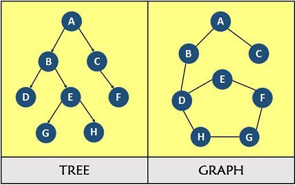
A graph G = (V, E) consists of a set of vertices (nodes) V and a set of edges E connecting pairs of vertices. Graphs are one of the most versatile data structures in computer science, used to model networks, dependencies, maps, social connections, and compilers.
| Type | Description | Examples |
|---|---|---|
| Undirected | Edges have no direction; (u,v) = (v,u) | Road networks, social friendships |
| Directed (Digraph) | Edges have direction; (u,v) ≠ (v,u) | Web links, task dependencies |
| Weighted | Each edge has a numeric weight/cost | Road distances, network latency |
| Unweighted | All edges treated as equal (weight=1) | Social networks, maze paths |
| Connected | Every vertex is reachable from every other vertex | Connected network infrastructure |
| DAG | Directed Acyclic Graph — no cycles | Build systems, course prerequisites |
| Complete | Every pair of vertices is connected by an edge | K-complete networks |
Important Terms
- Degree: Number of edges incident to a vertex. In directed graphs: in-degree (edges entering) and out-degree (edges leaving).
- Path: A sequence of vertices where consecutive pairs are connected by edges. A simple path visits no vertex twice.
- Cycle: A path that begins and ends at the same vertex.
- Connected Component: A maximal set of vertices such that there is a path between every pair.
- Spanning Tree: A subgraph that includes all vertices and is a tree (connected, acyclic). Has exactly |V|−1 edges.
§ 6.2 — Graph Representations
Graph Representations
How a graph is stored in memory significantly affects the time and space complexity of graph algorithms. The two primary representations are Adjacency Matrix and Adjacency List.
1. Adjacency Matrix
An n×n matrix A where A[i][j] = 1 (or weight w) if edge (i,j) exists, else 0.
Graph:  1──2        Matrix:
        |  |          1  2  3  4
        3──4        1[0, 1, 1, 0]
                    2[1, 0, 0, 1]
Edges: (1,2),(1,3), 3[1, 0, 0, 1]
       (2,4),(3,4)  4[0, 1, 1, 0]
PYTHON — Adjacency Matrix
class GraphMatrix:
    def __init__(self, n):
        self.n = n
        # n×n matrix initialized to 0
        self.adj = [[0]*n for _ in range(n)]

    def add_edge(self, u, v, w=1):
        self.adj[u][v] = w
        self.adj[v][u] = w   # remove for directed graph

    def has_edge(self, u, v):
        return self.adj[u][v] != 0   # O(1) lookup!
2. Adjacency List
An array of lists where adj[v] contains all vertices adjacent to v. Preferred for sparse graphs where |E| << |V|².
adj[1] → [2, 3]
adj[2] → [1, 4]
adj[3] → [1, 4]
adj[4] → [2, 3]
PYTHON — Adjacency List
from collections import defaultdict

class GraphList:
    def __init__(self):
        self.adj = defaultdict(list)

    def add_edge(self, u, v, w=1):
        self.adj[u].append((v, w))
        self.adj[v].append((u, w))   # undirected

    def neighbours(self, v):
        return self.adj[v]   # O(1) access to neighbour list
Efficiency Comparison
| Operation | Adjacency Matrix | Adjacency List |
|---|---|---|
| Space | O(V²) | O(V + E) |
| Add edge | O(1) | O(1) |
| Check if (u,v) exists | O(1) | O(degree(u)) |
| Find all neighbours of v | O(V) | O(degree(v)) |
| Best for | Dense graphs (E ≈ V²) | Sparse graphs (E << V²) |
Choose Adjacency List for most real-world sparse graphs (social networks, roads, web graphs). Choose Adjacency Matrix only for dense graphs or when O(1) edge-existence queries are critical.
§ 6.3 — Breadth-First Search (BFS)
Breadth-First Search (BFS)
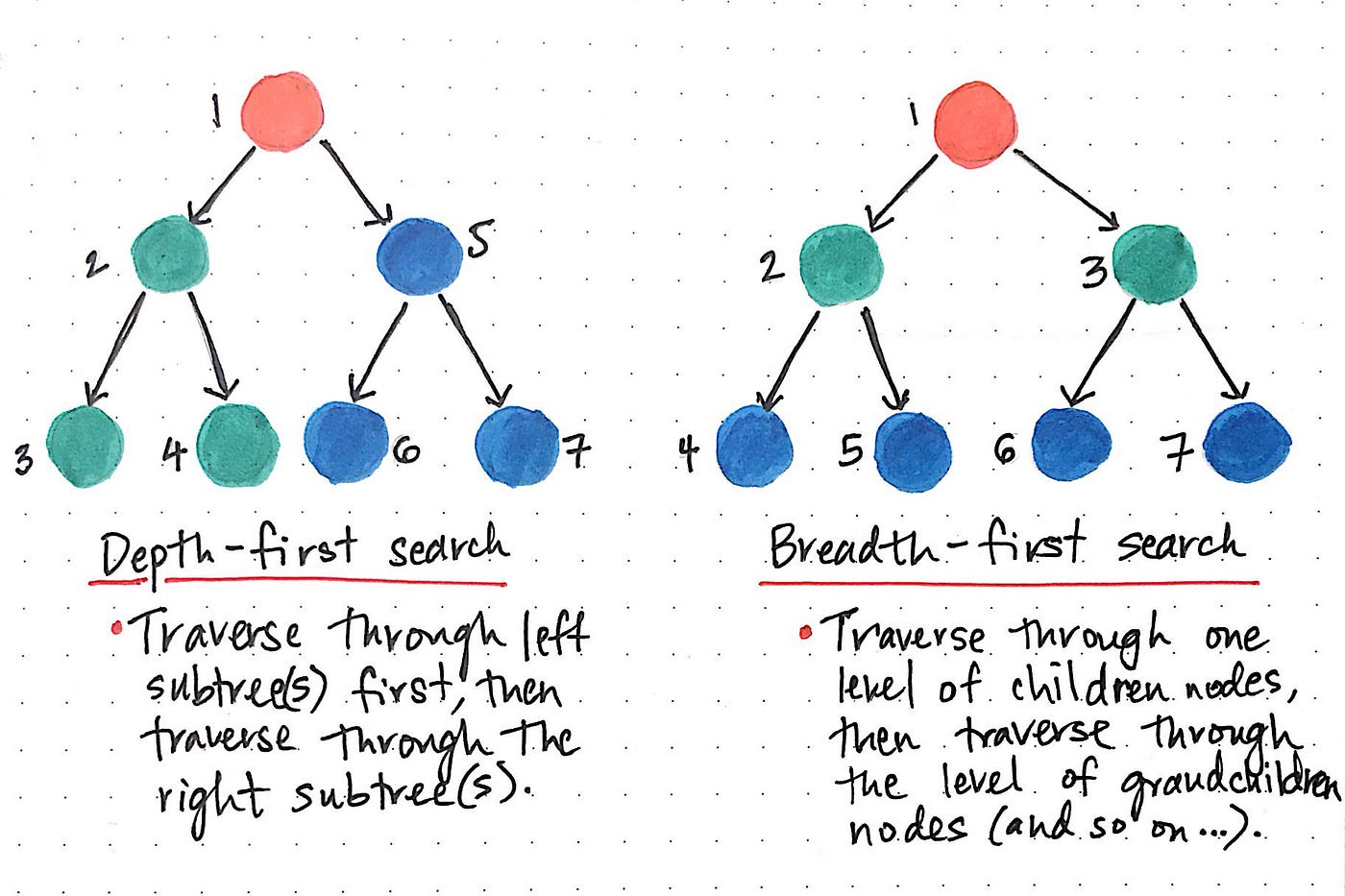
Breadth-First Search explores a graph level-by-level from a source vertex s, visiting all neighbours at distance k before any vertex at distance k+1. It uses a queue (FIFO) to ensure this ordering.
- Initialize: color all vertices WHITE, distance[s] = 0, enqueue s, color[s] = GRAY.
- While queue is not empty:
- Dequeue vertex u from front of queue.
- For each neighbour v of u:
- If color[v] == WHITE: set color[v] = GRAY, dist[v] = dist[u]+1, parent[v] = u, enqueue v.
- Set color[u] = BLACK.
PYTHON — Breadth-First Search
from collections import deque

def bfs(graph, start):
    visited = set()
    dist = {start: 0}
    parent = {start: None}
    queue = deque([start])
    visited.add(start)
    order = []

    while queue:
        u = queue.popleft()       # FIFO dequeue
        order.append(u)

        for v in graph[u]:
            if v not in visited:
                visited.add(v)
                dist[v] = dist[u] + 1
                parent[v] = u
                queue.append(v)   # enqueue neighbour
    return order, dist, parent
Graph Edges: A-B, A-C, B-D, B-E, C-F

Step 1: Queue=[A],    Visited={A}
Step 2: Process A  → Enqueue B,C.  Queue=[B,C],   dist: B=1,C=1
Step 3: Process B  → Enqueue D,E.  Queue=[C,D,E], dist: D=2,E=2
Step 4: Process C  → Enqueue F.    Queue=[D,E,F], dist: F=2
Step 5: Process D  → no new.       Queue=[E,F]
Step 6: Process E  → no new.       Queue=[F]
Step 7: Process F  → no new.       Queue=[]

BFS Order: A → B → C → D → E → F
Shortest path (A→F): A → C → F (distance = 2)
§ 6.4 — Depth-First Search (DFS)
Depth-First Search (DFS)
Depth-First Search explores a graph by going as deep as possible along each branch before backtracking. It uses a stack (implicit via recursion) and timestamps vertices to record discovery and finish times — which are vital for topological sort and strongly connected components.
- Initialize all vertices as WHITE, time = 0.
- For each vertex u in V: if u is WHITE, call DFS-VISIT(u).
- DFS-VISIT(u):
- time++; d[u] = time; color[u] = GRAY
- For each neighbour v of u: if v is WHITE, set parent[v]=u and DFS-VISIT(v).
- time++; f[u] = time; color[u] = BLACK
PYTHON — Depth-First Search (Recursive)
def dfs_recursive(graph, start, visited=None):
    if visited is None:
        visited = set()
    visited.add(start)
    print(start, end=' ')   # process vertex

    for neighbour in graph[start]:
        if neighbour not in visited:
            dfs_recursive(graph, neighbour, visited)
    return visited
DFS Edge Classification
| Edge Type | Condition (exploring u→v) | Meaning |
|---|---|---|
| Tree Edge | v is WHITE when discovered via u | Forms the DFS spanning tree |
| Back Edge | v is GRAY (ancestor of u) | Indicates a cycle in directed graph |
| Forward Edge | v is BLACK & d[u] < d[v] | Shortcut to descendant |
| Cross Edge | v is BLACK & d[u] > d[v] | Between different subtrees |
BFS Applications
- Shortest path (unweighted)
- Level-order traversal
- Finding connected components
DFS Applications
- Topological sorting of DAGs
- Cycle detection
- Finding strongly connected components
§ 6.5 & 6.6 — Minimum Spanning Tree & Kruskal's Algorithm
Minimum Spanning Tree (MST) & Kruskal's Algorithm
Kruskal's Algorithm builds the MST by greedily adding the minimum-weight edge that does not create a cycle. It processes edges in sorted order and uses a Union-Find (Disjoint Set Union) data structure to detect cycles.
- Sort all edges in non-decreasing order of weight.
- Initialize each vertex as its own component (n singleton sets).
- For each edge (u, v) in sorted order:
- If u and v are in different components: add edge to MST, UNION(u, v).
- Else: discard edge (would create a cycle).
- Stop when MST has V−1 edges.
PYTHON — Kruskal's Algorithm with Union-Find
class UnionFind:
    def __init__(self, n):
        self.parent = list(range(n))
        self.rank = [0] * n

    def find(self, x):   # Path compression
        if self.parent[x] != x:
            self.parent[x] = self.find(self.parent[x])
        return self.parent[x]

    def union(self, x, y):   # Union by rank
        rx, ry = self.find(x), self.find(y)
        if rx == ry: return False
        if self.rank[rx] < self.rank[ry]:
            rx, ry = ry, rx
        self.parent[ry] = rx
        if self.rank[rx] == self.rank[ry]:
            self.rank[rx] += 1
        return True

def kruskal(n, edges):
    edges.sort()   # O(E log E)
    uf = UnionFind(n)
    mst = []; total_weight = 0

    for w, u, v in edges:
        if uf.union(u, v):
            mst.append((u, v, w))
            total_weight += w
            if len(mst) == n - 1: break
    return mst, total_weight

§ 6.7 — Prim's Algorithm
Prim's Algorithm
Prim's Algorithm builds the MST by greedily growing a single connected tree from an arbitrary starting vertex. It adds the minimum-weight edge connecting the current MST to a vertex not yet in it. Uses a priority queue (min-heap).
- Initialize: key[v] = ∞, key[start] = 0, parent[start] = NULL.
- Insert all vertices into a min-priority queue Q keyed by key[v].
- While Q is not empty:
- Extract u = vertex with minimum key from Q.
- For each neighbour v of u:
- If v is still in Q AND weight(u,v) < key[v]: update key[v] = weight(u,v), parent[v] = u.
PYTHON — Prim's Algorithm (Min-Heap)
import heapq

def prim(graph, start=0):
    n = len(graph)
    in_mst = [False] * n
    key = [float('inf')] * n
    parent = [-1] * n
    key[start] = 0
    heap = [(0, start)]
    mst_edges = []; total = 0

    while heap:
        w, u = heapq.heappop(heap)
        if in_mst[u]: continue
        in_mst[u] = True

        if parent[u] != -1:
            mst_edges.append((parent[u], u, w))
            total += w

        for v, edge_w in graph[u]:
            if not in_mst[v] and edge_w < key[v]:
                key[v] = edge_w
                parent[v] = u
                heapq.heappush(heap, (key[v], v))
    return mst_edges, total
| Aspect | Kruskal's | Prim's |
|---|---|---|
| Approach | Edge-based: safe edge globally | Vertex-based: expand tree |
| Data Structure | Union-Find | Priority Queue |
| Best for | Sparse graphs | Dense graphs |
§ 6.8 — Dijkstra's Algorithm (SSSP)
Dijkstra's Algorithm (Single-Source Shortest Path)
Dijkstra's Algorithm solves the Single-Source Shortest Path (SSSP) problem for graphs with non-negative edge weights.
Important Constraint: Dijkstra's algorithm requires non-negative edge weights. For graphs with negative weights, use the Bellman-Ford algorithm.
- Initialize: dist[s] = 0, dist[v] = ∞. Insert all vertices into min-priority queue.
- While priority queue is not empty:
- Extract u = vertex with minimum dist[u].
- Relaxation: For each neighbour v of u: if dist[u] + w(u,v) < dist[v], update dist[v] = dist[u] + w(u,v). Decrease-key v in priority queue.
PYTHON — Dijkstra's Algorithm (Min-Heap)
import heapq

def dijkstra(graph, source):
    dist = {v: float('inf') for v in graph}
    dist[source] = 0
    parent = {v: None for v in graph}
    settled = set()
    pq = [(0, source)]

    while pq:
        d, u = heapq.heappop(pq)
        if u in settled: continue
        settled.add(u)

        for v, w in graph[u]:
            if v in settled: continue
            new_dist = dist[u] + w  # RELAXATION
            if new_dist < dist[v]:
                dist[v] = new_dist
                parent[v] = u
                heapq.heappush(pq, (new_dist, v))
    return dist, parent
§ 6.9 — Floyd-Warshall Algorithm (APSP)
Floyd-Warshall Algorithm (All-Pairs Shortest Paths)
The Floyd-Warshall Algorithm solves the All-Pairs Shortest Path (APSP) problem. It works on graphs with negative edge weights (but not negative cycles) and uses a classic DP approach.
PYTHON — Floyd-Warshall Algorithm
def floyd_warshall(n, edges):
    INF = float('inf')
    d = [[INF]*n for _ in range(n)]

    for i in range(n): d[i][i] = 0
    for u, v, w in edges: d[u][v] = w

    for k in range(n):
        for i in range(n):
            for j in range(n):
                if d[i][k] + d[k][j] < d[i][j]:
                    d[i][j] = d[i][k] + d[k][j]

    # Detect negative cycles
    for i in range(n):
        if d[i][i] < 0:
            raise ValueError("Negative cycle detected!")
    return d
| Algorithm | Problem | Weights | Time | Best For |
|---|---|---|---|---|
| BFS | SSSP | Unweighted only | O(V+E) | Unweighted sparse graphs |
| Dijkstra's | SSSP | Non-negative only | O((V+E) log V) | Weighted graphs, GPS |
| Bellman-Ford | SSSP | Negative allowed | O(VE) | Negative weights, detect neg cycles |
| Floyd-Warshall | APSP | Negative allowed | O(V³) | All pairs, dense graphs |
- Graph Representation: Adjacency List (best for sparse) vs Adjacency Matrix (best for dense).
- BFS & DFS: BFS (Queue) for unweighted shortest paths. DFS (Stack) for topological sort, cycles. Both O(V+E).
- MST (Kruskal & Prim): Kruskal sorts edges (Union-Find). Prim grows tree from a vertex (Min-Heap).
- Shortest Paths (Dijkstra & Floyd-Warshall): Dijkstra (SSSP, greedy, no negative edges). Floyd-Warshall (APSP, DP O(V³), negative edges allowed).